[影像處理] 找尋圖像邊緣

這邊我們將介紹幾種不同的方法用來找尋圖像的邊緣：
1. 高頻濾波法
2. 低頻濾波法
3. Edge filter
4. Canny edge detection
5. 富利略轉換
其中效果最好的是Canny edge detection

import cv2

import numpy as np

from pylab import *

from scipy import ndimage

用高頻過濾器來找尋邊緣

In [3]:

#建立兩個 High pass filter, HPF 用來找尋邊緣(根據與周圍pixel訊號強度的差異)

kernel_3x3 = np.array([[-1, -1, -1],[-1, 8, -1],[-1, -1, -1]])

kernel_5x5 = np.array([[-1, -1, -1, -1, -1],

                       [-1, 1, 2, 1, -1],

                       [-1, 2, 4, 2, -1],

                       [-1, 1, 2, 1, -1],

                       [-1, -1, -1, -1, -1]])

In [4]:

# 顯示二維高頻濾波器

plt.plot()

imshow(kernel_3x3)

plt.show()

plt.plot()

imshow(kernel_5x5)

plt.show()

In [5]:

img = cv2.imread("../../elephant.jpg", 0)

# 使用scipy的ndimage的colvolve對影像img做kernel_3x3的convolution

k3 = ndimage.convolve(img, kernel_3x3)

# 使用scipy的ndimage的colvolve對影像img做kernel_5x5的convolution

k5 = ndimage.convolve(img, kernel_5x5)

cv2.imshow("3x3", k3)

cv2.imshow("5x5", k5)

cv2.waitKey()

cv2.destroyAllWindows()

用低頻過濾器來找尋邊緣

step 1: 先產生高斯模糊的影像 (高斯filter又稱為low pss filter (LPF), 因為它可以讓影像特徵變模糊)

In [6]:

blurred = cv2.GaussianBlur(img, (11,11), 0)

step 2: 將原圖減去高斯模糊的影像，這種做法有像是SIFT裡面找尋特徵點的作法(DOF)

In [7]:

g_hpf = img - blurred

cv2.imshow("g_hpf", g_hpf)

cv2.waitKey()

cv2.destroyAllWindows()

由結果論看，最後一種方法找尋邊緣的效果最好

邊緣過濾器 Edge filter

常用的三種 filter: Laplacian(), Sobel(), and Scharr(), Prewitt().

Prewitt filters:Sobel filters

把原圖對Dx filter 和 Dy filter做Convolution得到對0軸和1軸的微分圖

把每個pixel對0軸和1軸的微分圖平方相加開根號，得到梯度強度

每個pixel的最大強度變化的方向為

下圖 (a)處理前的照片 (b)對Dx做convolution (c)對Dy做Convolution (d)梯度強度

有時後Edge filter會把雜訊誤認成edge，因此可以先用blurring filters讓雜訊消除．

blurring filters： blur(),(simple average), medianBlur(), and GaussianBlur().

找尋edge的標準程序：

1. 使用medianBlur()移除雜訊
2. 把影像從BGR轉換成灰階
3. 使用Laplacian()尋找邊緣
4. 把影像inverse (黑變白，白變黑，Edge變黑)，並把數值normalize 到[0,1]
5. 把normalize後的結果與原圖相乘，使edge的影像變暗

In [8]:

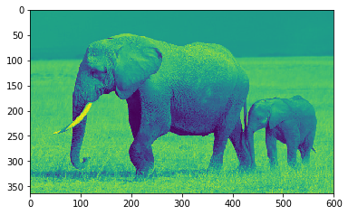
# step 1: 使用medianBlur()移除雜訊

blurKsize = 7

edgeKsize = 5

blurredSrc = cv2.medianBlur(img, blurKsize) #step 1

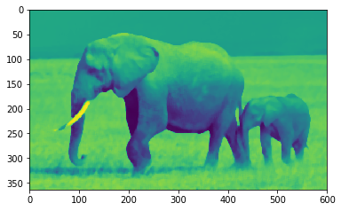
plt.plot()

imshow(img)

plt.show()

plt.plot()

imshow(blurredSrc)

plt.show()

In [9]:

# step 3: 使用Laplacian過濾器找尋邊緣

cv2.Laplacian(blurredSrc, cv2.CV_8U, blurredSrc, ksize = edgeKsize) #step 3

plt.plot()

imshow(blurredSrc)

plt.show()

In [11]:

#step 4: 把影像inverse (黑變白，白變黑，Edge變黑),並把數值normalize 到[0,1]

normalizedInverseAlpha = (1.0 / 255) * (255 - blurredSrc) 

plt.plot()

imshow(normalizedInverseAlpha)

plt.show()

In [15]:

#step 5: 把normalize後的結果與原圖相乘，使edge的影像變暗，這樣edge就會被描出來

img_after = img * normalizedInverseAlpha 

plt.plot()

imshow(img_after)

plt.show()

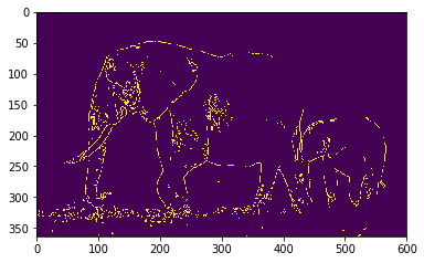
Canny edge detection

OpenCV提供了Canny找尋邊緣，由John F. Canny開發的演算法，只需要一行指令就可以得到edge Candy 演算法其實相當複雜，它包含了以下四個程序：

1. Denoises the image with a Gaussian filter
2. Calculates gradients
3. applies non maximum suppression (NMS) on edges, a double threshold on all the detected edges to eliminate false positives
4. Analyzes all the edges and their connection to each other to keep the real edges and discard the weak ones.

In [17]:

# %load canny.py

import cv2

import numpy as np

img = cv2.imread("../../elephant.jpg", 0)

cv2.imwrite("canny.jpg", cv2.Canny(img, 200, 300))

cv2.imshow("canny", cv2.imread("canny.jpg"))

cv2.waitKey()

cv2.destroyAllWindows()

In [18]:

imshow(cv2.Canny(img, 200, 300))

Out[18]:

<matplotlib.image.AxesImage at 0x1811bc4a90>

富利略轉換

用富利略轉換轉換把頻率低的訊號過濾掉 剩下平率高的訊號就是edge

In [19]:

import cv2

import numpy as np

from matplotlib import pyplot as plot

img = cv2.imread('../../elephant.jpg', 0)  #import第零個channel

img.shape

Out[19]:

(364, 600)

In [20]:

imshow(img)

Out[20]:

<matplotlib.image.AxesImage at 0x181e3729e8>

In [21]:

f = np.fft.fft2(img) #把圖片做Fourier轉換變成frequency domain

fshift = np.fft.fftshift(f) #把頻率為零的元素shift到spectrum正中間

magnitude_spectrum = 20 * np.log(np.abs(fshift)) #計算spectrum的強度

row, cols = img.shape

crow, ccol = row // 2, cols // 2 #計算中間位置

In [22]:

#把spectrum正中間附近30個pixel變成0 把[-30,30]頻率範圍的訊號強度變0

#把低頻的訊號過濾掉, 剩下高頻的訊號就會是edge

fshift[crow - 30: crow+30, ccol - 30: ccol + 30] = 0 

f_ishift = np.fft.ifftshift(fshift) #使用inverse fftshift恢復原來的頻率序列

img_back = np.fft.ifft2(f_ishift) #使用inverse fft把frequency domain轉換成pixel的domain

img_back = np.abs(img_back)#轉換成絕對值

plot.subplot(221), plot.imshow(img, cmap = "gray")

plot.title("Input"), plot.xticks([]), plot.yticks([])

plot.subplot(222), plot.imshow(magnitude_spectrum, cmap = "gray")

plot.title('magnitude_spectrum'), plot.xticks([]), plot.yticks([])

plot.subplot(223), plot.imshow(img_back, cmap = "gray")

plot.title("Input in JET"), plot.xticks([]), plot.yticks([])

plot.show()