[機器視覺] 尺度不變特徵轉換尋找特徵值原理(SIFT)

原文： https://towardsdatascience.com/sift-scale-invariant-feature-transform-c7233dc60f37

尺度不變特徵轉換(SIFT, Scale Invariant Feature Transform)是在2004年由David G. Lowe所提出，主要是用在影像特徵點萃取．其優點是所萃取 的特徵不易受到影像旋轉、縮放和灰度值差異而有所變化、具有良好特徵點選取與匹配，其匹配結果正確率較高並可消除影像處理中不確定性．目前常見的應用為全景圖的拼接：將圖片中相似特徵點的位置找出，並進行拼接，本篇文章將解釋SIFT的數學原理，並在最後我們會python將它實現在全景圖的拼接上．

SIFT演算法分成四個步驟：

1. 特徵值位置偵測(使用DoF)
2. 特徵點校正
3. 方向指定
4. 特徵描述

SIFT特徵萃取因為是尺度不變(Scale Invariance)，所以在做特徵萃取時效果比Harris好，Harris演算法常常在圖片放大時把corner特徵辨識為edge特徵，如下圖所示：

特徵值位置偵測(使用DoF)

SIFT如何達到尺度不變？？ 可以使用Laplacian of Gaussian(LoG)．

Laplacian of Gaussian(LoG)的操作方法如下：

1. 取一張圖，並用高斯濾鏡將它變模糊
2. 計算二次微分的總和(Laplacian)

得到特徵點(corner和edge)的位置．

從上面兩張圖可以得知，Edge的找法有兩種：

1. 高斯函數一次微分對圖片做convelution的最大值
2. 高斯函數二次微分對圖片做convelution的crossing 0點

找corner的方法如上：高斯內核(Gausian kernal)二次微分對圖片做convelution的極值(最大值或最小值)為corner的位置，偵測到的corner大小與高斯內核的大小相似．因此這個方法並非“尺度不變”．

若圖片中有一個半徑為8的corner，我們用σ=1,2,4,8,16的高斯內核二次微分分別對圖片做convelution．只有σ=8的高斯內核二次微分對圖片做convelution的極值才是corner的位置．且convolution值的大小會隨著σ的增加而變小，原因如下：σ越大下圖的紅色面積越小，所以convolution的值也就會越小．為了達到“尺度不變”，我們必須對comvolution的值乘上σ平方．數學證明參考以下連結．

經過σ平方的normalization後可以找到σ=8時會有極值，而這個物質就是corner的位置．

從上圖得知，實際上difference of Gausian (DoG)與Laplacian of Gausian (LoG)相似，實際上我們看可以用熱傳的方程式來證明DoF近似LoF：

左邊就是DoF；右邊就是LoF乘上σ平方．因此LoF可以用DoF取代，其運算流程如下圖所示．

特徵點校正

參考文章：N Campbell’s article

因為第一步驟的特徵點位置精確度與內核的選取數量(σ的數量)有關，因此我們要重新校正第一步驟搜尋到的特徵點位置．步驟如下：利用Taylor expansion fitting 3D quadratic surface (in x,y, and σ)找尋內差的最大或最小值．

z0是由[X,Y,σ]所組成的平面，z=[δx,δy,δσ]

把上面的式子對z做微分取零得到極值．

設定threshold，過濾掉threshold以下的特徵點位置．

方向指定

使用Histogram of Oriented Gradient (HOG)來定位．

特徵描述

[編碼器] 用深度學習神經網路製作自動編碼解碼器

用深度學習神經網路製作自動編碼解碼器

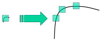
資料來源：https://medium.com/datadriveninvestor/deep-autoencoder-using-keras-b77cd3e8be95在這個案例中，我們將製作一個自動編碼器，他可以將圖片利用深度神經網路編碼成維度較小的資料，但這個維度較小的資料卻仍然保有原來資料的重要資訊，這些壓縮過的資料可以再經由解碼器還原成原來的資訊． 實作上我們將編碼器(encoder)接上解碼器(decoder)做訓練，編碼器：輸入資料為784維度的圖片資料，利用密集層(Dense layer)壓縮成32維度；解碼器：將32維度的資料利用密集層(Dense layer)展開成32維度．在訓練時，將編碼器和解碼器接在一起訓練，訓練時輸入資料為圖片28*28得陣列reshape成784維度的資料，輸出資料則和輸入資料相同，目的是為了訓練機器能夠在壓縮和展開資料時盡可能減少資料的損失．

編碼器應用範圍： 將重要資訊壓縮成較小的維度，並把不重要的資訊過濾掉(去除雜訊)．將encoder過的資訊拿去接其他神經網路能有效的提升訓練品質

這個案例中我們將實作mnist灰階數字圖片的編碼與解碼

from keras.datasets import mnist

from keras.layers import Input, Dense

from keras.models import Model

import numpy as np

import pandas as pd

import matplotlib.pyplot as plt

%matplotlib inline

#載入資料

(X_train, _), (X_test, _) = mnist.load_data()

X_train = X_train.astype('float32')/255

X_test = X_test.astype('float32')/255

X_train = X_train.reshape(len(X_train), np.prod(X_train.shape[1:]))

X_test = X_test.reshape(len(X_test), np.prod(X_test.shape[1:]))

print(X_train.shape)

print(X_test.shape)

(60000, 784)
(10000, 784)

# 輸入資料(輸入的資料為[0,1]之間的數字，維度是28*28=784維度的一維陣列(784,))
input_img= Input(shape=(784,))

#編碼器(都使用relu函數做非線性轉換)
encoded = Dense(units=128, activation='relu')(input_img)
encoded = Dense(units=64, activation='relu')(encoded)
encoded = Dense(units=32, activation='relu')(encoded)
#解碼器(輸出層使用sigmoid非線性函數將資料壓縮在[0,1]之間)
decoded = Dense(units=64, activation='relu')(encoded)
decoded = Dense(units=128, activation='relu')(decoded)
decoded = Dense(units=784, activation='sigmoid')(decoded)

#設定自動編碼器(編碼器＋解碼器)的輸入與輸出 autoencoder=Model(input_img, decoded)

#設定編碼器的輸入與輸出 encoder = Model(input_img, encoded)

#編碼器摘要 autoencoder.summary()

_________________________________________________________________
Layer (type)                 Output Shape              Param #   
=================================================================
input_1 (InputLayer)         (None, 784)               0         
_________________________________________________________________
dense_1 (Dense)              (None, 128)               100480    
_________________________________________________________________
dense_2 (Dense)              (None, 64)                8256      
_________________________________________________________________
dense_3 (Dense)              (None, 32)                2080      
_________________________________________________________________
dense_4 (Dense)              (None, 64)                2112      
_________________________________________________________________
dense_5 (Dense)              (None, 128)               8320      
_________________________________________________________________
dense_6 (Dense)              (None, 784)               101136    
=================================================================
Total params: 222,384
Trainable params: 222,384
Non-trainable params: 0
_________________________________________________________________

# 設定編碼器的訓練方法(optimizer, loss, metrics)
autoencoder.compile(optimizer='adam', loss='binary_crossentropy', metrics=['accuracy'])

# 訓練編碼器(輸入=輸出)

autoencoder.fit(X_train, X_train,

                epochs=50,

                batch_size=256,

                shuffle=True,

                validation_data=(X_test, X_test))

Epoch 47/50
60000/60000 [==============================] - 85s 1ms/step - loss: 0.0845 - acc: 0.8146 - val_loss: 0.0842 - val_acc: 0.8136
Epoch 48/50
60000/60000 [==============================] - 85s 1ms/step - loss: 0.0844 - acc: 0.8146 - val_loss: 0.0837 - val_acc: 0.8137
Epoch 49/50
60000/60000 [==============================] - 79s 1ms/step - loss: 0.0842 - acc: 0.8146 - val_loss: 0.0838 - val_acc: 0.8137
Epoch 50/50
60000/60000 [==============================] - 80s 1ms/step - loss: 0.0841 - acc: 0.8146 - val_loss: 0.0834 - val_acc: 0.8137

# 編碼資料
encoded_imgs = encoder.predict(X_test)

# 編碼＋解碼資料
predicted = autoencoder.predict(X_test)

# 視覺化 編碼前資料，編碼後資料，解碼後資料
plt.figure(figsize=(40, 4))
for i in range(10):
    # display original images
    ax = plt.subplot(3, 20, i + 1)
    plt.imshow(X_test[i].reshape(28, 28))
    plt.gray()
    ax.get_xaxis().set_visible(False)
    ax.get_yaxis().set_visible(False)
    
    # display encoded images
    ax = plt.subplot(3, 20, i + 1 + 20)
    plt.imshow(encoded_imgs[i].reshape(8,4))
    plt.gray()
    ax.get_xaxis().set_visible(False)
    ax.get_yaxis().set_visible(False)
    # display reconstructed images
    ax = plt.subplot(3, 20, 2*20 +i+ 1)
    plt.imshow(predicted[i].reshape(28, 28))
    plt.gray()
    ax.get_xaxis().set_visible(False)
    ax.get_yaxis().set_visible(False)

驗證編碼器是否具備去除圖片雜訊的功能



#loading only images and not their labels
(X_train, _), (X_test, _) = mnist.load_data()

X_train = X_train.astype('float32')/255
X_test = X_test.astype('float32')/255

X_train = X_train.reshape(len(X_train), np.prod(X_train.shape[1:]))
X_test = X_test.reshape(len(X_test), np.prod(X_test.shape[1:]))

#製作雜訊
X_train_noisy = X_train + np.random.normal(loc=0.0, scale=0.5, size=X_train.shape)
X_train_noisy = np.clip(X_train_noisy, 0., 1.)
X_test_noisy = X_test + np.random.normal(loc=0.0, scale=0.5, size=X_test.shape)
X_test_noisy = np.clip(X_test_noisy, 0., 1.)
print(X_train_noisy.shape)
print(X_test_noisy.shape)



(60000, 784)
(10000, 784)

plt.imshow(X_train_noisy[0].reshape(28,28))

#Input image
input_img= Input(shape=(784,))
# encoded and decoded layer for the autoencoder
encoded = Dense(units=128, activation='relu')(input_img)
encoded = Dense(units=64, activation='relu')(encoded)
encoded = Dense(units=32, activation='relu')(encoded)
decoded = Dense(units=64, activation='relu')(encoded)
decoded = Dense(units=128, activation='relu')(decoded)
decoded = Dense(units=784, activation='sigmoid')(decoded)
# Building autoencoder
autoencoder=Model(input_img, decoded)
#extracting encoder
encoder = Model(input_img, encoded)
# compiling the autoencoder
autoencoder.compile(optimizer='adadelta', loss='binary_crossentropy', metrics=['accuracy'])

# Fitting the noise trained data to the autoencoder 
autoencoder.fit(X_train_noisy, X_train_noisy,
                epochs=100,
                batch_size=256,
                shuffle=True,
                validation_data=(X_test_noisy, X_test_noisy))

# reconstructing the image from autoencoder and encoder
encoded_imgs = encoder.predict(X_test_noisy)
predicted = autoencoder.predict(X_test_noisy)

# plotting the noised image, encoded image and the reconstructed image
plt.figure(figsize=(40, 4))
for i in range(10):
# display original images
    
    ax = plt.subplot(4, 20, i + 1)
    plt.imshow(X_test[i].reshape(28, 28))
    plt.gray()
    ax.get_xaxis().set_visible(False)
    ax.get_yaxis().set_visible(False)
    
# display noised images
    ax = plt.subplot(4, 20, i + 1+20)
    plt.imshow(X_test_noisy[i].reshape(28, 28))
    plt.gray()
    ax.get_xaxis().set_visible(False)
    ax.get_yaxis().set_visible(False)
# display encoded images    
    ax = plt.subplot(4, 20, 2*20+i + 1 )
    plt.imshow(encoded_imgs[i].reshape(8,4))
    plt.gray()
    ax.get_xaxis().set_visible(False)
    ax.get_yaxis().set_visible(False)
# display reconstruction images
    ax = plt.subplot(4, 20, 3*20 +i+ 1)
    plt.imshow(predicted[i].reshape(28, 28))
    plt.gray()
    ax.get_xaxis().set_visible(False)
    ax.get_yaxis().set_visible(False)
    
    
plt.show()

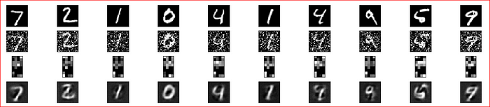
編碼器的確可以把雜訊過濾掉僅留下重要的資訊