與時間序列相關的預測問題非常多,例如: 選舉預測,供應鏈預測,運算預測,股票預測,GDP,通膨預測,健康預測,地震預報...等

時間序列資料的預測方法:
時間序列資料預測的方法有以下幾種:
- 線性統計學(MA,ARIMA, SARIMA...etc)
- 非線性統計學(NAR...etc)
- 機器學習 (SVM...etc)
- 深度學習(RNN, LSTM,GRU...etc)

這邊介紹如何使用ARIMA model:
Auto Regressive Moving Average Model (ARIMA)
使用在非靜態(non-stationary)
參數:
p: order of Auto regression terms (number of time-step lags)
q: order of Moving average terms
d: order of differencing for attaining stationarity
使用步驟:
Step 1. 畫出資料,檢查資料是否有週期趨勢, 檢查是否有NaN,ARIMA無法處理NaN資料
Step 1. 畫出資料,檢查資料是否有週期趨勢, 檢查是否有NaN,ARIMA無法處理NaN資料
Step 2. 使用Augmented Dickey Fuller Test(adfuller())函數確認資料是否為靜態,若為靜態使用ARMA, 若不為靜態則使用ARIMA
Step 3. 執行ETS Decomposition (seasonal_decompose())函數檢查資料是否有週期性,若週期性訊號相較於整體訊號微小則可以使用非週期性的ARIMA模型(如下圖)

ARIMA的參數
ACF - can be used to determine the MA order (q).
PACF - can be used to determine the AR order (p).
若資料的週期性訊號明顯,則需使用週期性ARIMA 或 SARIMA
Step 4. 使用自動金字塔ARIMA(automated pyramid ARIMA)函數(auto_arima())決定ARIMA的(p,d,q)參數與SARIMA的(p, d, q, P, D, Q)
Step 5. 將資料分成訓練和測試資料
Step 6. 使用ARIMA()函數來fitting, 將第四步驟得到的的 p,d,q 參數設定進ARIMA
Step 7: 使用predict()函數來測試模型
Step 8: 重複訓練
案例: 用ARIMA模型預測北京PM2.5
import pandas as pd
from pandas.plotting import register_matplotlib_converters
import numpy as np
import statsmodels.api as sm
import matplotlib.pyplot as plt
from pylab import rcParams
import itertools
from pandas import DataFrame
import math
from sklearn.metrics import mean_squared_error
dataset = pd.read_csv('PRSA_data_2010.1.1-2014.12.31.csv')
# Transformation for the date
dataset['Timestamp'] = dataset['year'].map(str) + "/" + dataset['month'].map(str) + "/" + dataset['day'].map(str) + ' ' + dataset['hour'].map(str) + ":" + "00:00"
dataset['Timestamp'] = pd.to_datetime(dataset['Timestamp'])
dataset = dataset.set_index('Timestamp')
# Drop the columns that are not going to be used
dataset = dataset.drop(['No',
'year',
'month',
'day',
'hour',
'DEWP',
'TEMP',
'PRES',
'cbwd',
'Iws',
'Is',
'Ir'], axis=1)
dataset = dataset.dropna()
Step 1. 畫出資料,檢查資料是否有週期趨勢
register_matplotlib_converters()
plt.figure(figsize=(20,6))
plt.plot(dataset.index, dataset['pm2.5'])
plt.title("Levels of PM2.5 particles in Beijing")
plt.ylabel("PM2.5 concentration (ug/m^3)")
plt.show()

Grouping by different frames of time
weekly = dataset['pm2.5'].resample('W').mean()
plt.figure(figsize=(20,7))
plt.plot(weekly)
plt.title("The weekly average of PM2.5 concentration")
plt.ylabel("PM2.5 particles")
plt.grid()
plt.show()

monthly = dataset['pm2.5'].resample('M').mean()
plt.figure(figsize=(20,7))
plt.plot(monthly)
plt.title("The monthly average of PM2.5 concentration")
plt.ylabel("PM2.5 particles")
plt.grid()
plt.show()

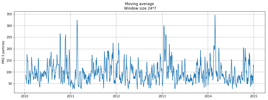
移動平均 Moving average
movingAverage = dataset['pm2.5'].rolling(window=24).mean()
plt.figure(figsize=(15,5))
plt.title("Moving average\n Window size 24, equivalent to one day")
plt.ylabel("PM2.5 particles")
plt.plot(movingAverage,label="Rolling mean trend")
plt.grid(True)

movingAverage = dataset['pm2.5'].rolling(window=(24*7)).mean()
plt.figure(figsize=(15,5))
plt.title("Moving average\n Window size 24*7")
plt.ylabel("PM2.5 particles")
plt.plot(movingAverage,label="Rolling mean trend")
plt.grid(True)
movingAverage = dataset['pm2.5'].rolling(window=(24*7*30)).mean()
plt.figure(figsize=(15,5))
plt.title("Moving average\n Window size 5.040, equivalent to one month")
plt.plot(movingAverage,label="Rolling mean trend")
plt.ylabel("PM2.5 particles")
plt.grid(True)
plt.show()

Getting closer to the last weeks
last_weeks = dataset.loc['2014-12':'2014']
plt.figure(figsize=(15,5))
plt.title("PM2.5 particules in December 2014")
plt.ylabel("PM2.5 particles")
plt.plot(last_weeks)

plt.hist(last_weeks['pm2.5'])
(array([395., 94., 81., 46., 30., 22., 14., 18., 15., 1.]),
array([ 4., 48., 92., 136., 180., 224., 268., 312., 356., 400., 444.]),
<a list of 10 Patch objects>)

Step 2. 使用Augmented Dickey Fuller Test(adfuller())函數確認資料是否為靜態
from statsmodels.tsa.stattools import adfuller
#Perform Dickey-Fuller test:
print ('Results of Dickey-Fuller Test:')
dftest = adfuller(last_weeks['pm2.5'], autolag='AIC')
dfoutput = pd.Series(dftest[0:4], index=['Test Statistic','p-value','#Lags Used','Number of Observations Used'])
for key,value in dftest[4].items():
dfoutput['Critical Value (%s)'%key] = value
print (dfoutput)
p_value = dftest[1]
if p_value <= 0.01:
print("\nData is stationary")
else:
print("\n Data is non-stationary ")
Results of Dickey-Fuller Test:
Test Statistic -4.990870
p-value 0.000023
#Lags Used 2.000000
Number of Observations Used 713.000000
Critical Value (10%) -2.568933
Critical Value (1%) -3.439555
Critical Value (5%) -2.865602
dtype: float64
Data is stationary
很幸運的,資料為靜態的,我們可以直接使用ARIMA模型
Step 5. 將資料分成訓練和測試資料
train_dataset = last_weeks['2014-12': '2014-12-29']
test_dataset = last_weeks['2014-12-30': '2014']
檢查時間序列的相關性
使用Autocorrelation Function (ACF) 和 Partial Autocorrelation Function (PACF)
fig = plt.figure(figsize=(12,8))
ax1 = fig.add_subplot(211)
fig = sm.graphics.tsa.plot_acf(train_dataset['pm2.5'], lags=40, ax=ax1)
ax2 = fig.add_subplot(212)
fig = sm.graphics.tsa.plot_pacf(train_dataset['pm2.5'], lags=40, ax=ax2)

Step 6. 使用ARIMA()函數來fitting
from statsmodels.tsa.arima_model import ARIMA
model = ARIMA(train_dataset, order=(3,0,0))
model_fit = model.fit(disp=0)
print(model_fit.summary())
ARMA Model Results
==============================================================================
Dep. Variable: pm2.5 No. Observations: 668
Model: ARMA(3, 0) Log Likelihood -3098.247
Method: css-mle S.D. of innovations 24.956
Date: Sun, 14 Jul 2019 AIC 6206.495
Time: 03:12:58 BIC 6229.016
Sample: 12-01-2014 HQIC 6215.219
- 12-29-2014
===============================================================================
coef std err z P>|z| [0.025 0.975]
-------------------------------------------------------------------------------
const 83.2433 18.867 4.412 0.000 46.264 120.222
ar.L1.pm2.5 1.1707 0.039 30.407 0.000 1.095 1.246
ar.L2.pm2.5 -0.1370 0.059 -2.310 0.021 -0.253 -0.021
ar.L3.pm2.5 -0.0840 0.039 -2.177 0.030 -0.160 -0.008
Roots
=============================================================================
Real Imaginary Modulus Frequency
-----------------------------------------------------------------------------
AR.1 1.0820 +0.0000j 1.0820 0.0000
AR.2 2.2279 +0.0000j 2.2279 0.0000
AR.3 -4.9414 +0.0000j 4.9414 0.5000
-----------------------------------------------------------------------------
residuals = DataFrame(model_fit.resid)
residuals.plot()
plt.show()

residuals.plot(kind='kde')
plt.xlim([-100.0, 100.0])
plt.show()
print(residuals.describe())

count 668.000000
mean 0.012302
std 25.009394
min -206.193511
25% -6.264588
50% -1.666555
75% 7.713271
max 173.018662
Step 7: 使用predict()函數來測試模型
test = test_dataset.values
X = train_dataset.values
size = len(X)
history = [x for x in X]
predictions = list()
for t in range(len(test)):
model = ARIMA(history, order=(3,0,0))
model_fit = model.fit(disp=0)
output = model_fit.forecast()
yhat = output[0]
predictions.append(yhat)
obs = test[t]
history.append(obs)
print('predicted=%f, expected=%f' % (yhat, obs))
error = mean_squared_error(test, predictions)
print('Test MSE: %.3f' % error)
predicted=157.112900, expected=189.000000
predicted=189.929226, expected=97.000000
predicted=79.233638, expected=81.000000
predicted=69.324655, expected=28.000000
predicted=17.842556, expected=25.000000
predicted=22.027169, expected=9.000000
predicted=9.003651, expected=9.000000
predicted=11.096946, expected=13.000000
predicted=17.344109, expected=17.000000
predicted=21.536121, expected=16.000000
predicted=19.514494, expected=25.000000
predicted=29.680554, expected=48.000000
predicted=55.500414, expected=49.000000
predicted=53.157692, expected=73.000000
predicted=78.621660, expected=65.000000
predicted=66.562004, expected=55.000000
predicted=53.407227, expected=60.000000
predicted=61.132516, expected=63.000000
predicted=65.061522, expected=79.000000
predicted=82.800462, expected=35.000000
predicted=29.699352, expected=26.000000
predicted=22.490444, expected=20.000000
predicted=20.937708, expected=8.000000
predicted=8.572365, expected=16.000000
predicted=19.778056, expected=10.000000
predicted=13.140365, expected=11.000000
predicted=14.142651, expected=20.000000
predicted=25.074882, expected=9.000000
predicted=11.217382, expected=8.000000
predicted=10.347984, expected=9.000000
predicted=12.718046, expected=8.000000
predicted=11.540478, expected=8.000000
predicted=11.541062, expected=8.000000
predicted=11.633717, expected=8.000000
predicted=11.625385, expected=7.000000
predicted=10.456640, expected=12.000000
predicted=16.361236, expected=17.000000
predicted=21.706934, expected=11.000000
predicted=13.685557, expected=9.000000
predicted=11.514237, expected=11.000000
predicted=14.649415, expected=8.000000
predicted=11.141699, expected=9.000000
predicted=12.423357, expected=10.000000
predicted=13.768003, expected=8.000000
predicted=11.227813, expected=10.000000
predicted=13.661358, expected=10.000000
predicted=13.634794, expected=8.000000
predicted=11.105488, expected=12.000000
Test MSE: 338.965
plt.figure(figsize=(20,7))
plt.plot(test, label='Test')
plt.plot(predictions, label='Predictions', color='red')
plt.legend(prop={'size': 15})
plt.show()

計算測試資料誤差值
error = mean_squared_error(test, predictions)
print('Test Mean Squared Error(MSE): %.3f' % error)
下面我們將比較統計學上的ARIMA model與深度學習的RNN model的預測準確度
from sklearn.preprocessing import MinMaxScaler
normalize = MinMaxScaler(feature_range = (0, 1))
train_dataset = normalize.fit_transform(train_dataset)
plt.plot(train_dataset)

X_train = []
y_train = []
for i in range(168, train_dataset.shape[0]):
X_train.append(train_dataset[i-168:i, 0])
y_train.append(train_dataset[i, 0])
X_train, y_train = np.array(X_train), np.array(y_train)
X_train = np.reshape(X_train, (X_train.shape[0], X_train.shape[1], 1))
# Importing the Keras libraries and packages
from keras.models import Sequential
from keras.layers import Dense
from keras.layers import LSTM
from keras.layers import Dropout
# Initialising the RNN
regressor = Sequential()
# Adding the first LSTM layer and some Dropout regularisation
regressor.add(LSTM(units = 10, return_sequences = True, input_shape = (X_train.shape[1], 1)))
regressor.add(Dropout(0.4))
# Adding a second LSTM layer and some Dropout regularisation
regressor.add(LSTM(units = 20, return_sequences = True))
regressor.add(Dropout(0.4))
# Adding a third LSTM layer and some Dropout regularisation
regressor.add(LSTM(units = 30, return_sequences = True))
regressor.add(Dropout(0.4))
# Adding a fourth LSTM layer and some Dropout regularisation
regressor.add(LSTM(units = 20, return_sequences = True))
regressor.add(Dropout(0.4))
# Adding a fiveth LSTM layer and some Dropout regularisation
regressor.add(LSTM(units = 10))
regressor.add(Dropout(0.4))
# Adding the output layer
regressor.add(Dense(units = 1))
# Compiling the RNN
regressor.compile(optimizer = 'adam', loss = 'mean_squared_error')
regressor.fit(X_train, y_train, epochs = 100, batch_size = 32)
Epoch 87/100
500/500 [==============================] - 59s 118ms/step - loss: 0.0142
Epoch 88/100
500/500 [==============================] - 54s 109ms/step - loss: 0.0138
Epoch 89/100
500/500 [==============================] - 63s 126ms/step - loss: 0.0145
Epoch 90/100
500/500 [==============================] - 55s 109ms/step - loss: 0.0130
Epoch 91/100
500/500 [==============================] - 63s 125ms/step - loss: 0.0142
Epoch 92/100
500/500 [==============================] - 61s 121ms/step - loss: 0.0131
Epoch 93/100
500/500 [==============================] - 57s 114ms/step - loss: 0.0127
Epoch 94/100
500/500 [==============================] - 74s 147ms/step - loss: 0.0145
Epoch 95/100
500/500 [==============================] - 62s 124ms/step - loss: 0.0127
Epoch 96/100
500/500 [==============================] - 43s 86ms/step - loss: 0.0139
Epoch 97/100
500/500 [==============================] - 34s 67ms/step - loss: 0.0127
Epoch 98/100
500/500 [==============================] - 39s 77ms/step - loss: 0.0144
Epoch 99/100
500/500 [==============================] - 32s 64ms/step - loss: 0.0145
Epoch 100/100
500/500 [==============================] - 32s 65ms/step - loss: 0.0123
regressor.save('PM2d5.h5')
inputs = last_weeks[len(last_weeks) - len(test_dataset) - 168 :].values
inputs = inputs.reshape(-1,1)
inputs = normalize.transform(inputs)
X_test = []
for i in range(168, len(inputs)):
X_test.append(inputs[i-168:i, 0])
X_test = np.array(X_test)
X_test = np.reshape(X_test, (X_test.shape[0], X_test.shape[1], 1))
predicted = regressor.predict(X_test)
predicted = normalize.inverse_transform(predicted)
# Visualising the results
plt.figure(figsize=(20,7))
plt.plot(test_dataset['pm2.5'].values, color = 'red', label = 'Real Values')
plt.plot(predicted, color = 'blue', label = 'Predicted Values')
plt.title('Contamination prediction')
plt.xlabel('Time')
plt.ylabel('PM2.5')
plt.legend()
plt.show()

mean_squared_error(test_dataset['pm2.5'].values, predicted)
839.7245282817906
深度學習RNN的誤差值是統計學ARIMA的2.5倍,在這個案例上深度學習不但需要訓練的時間長,預測的準確度也遠不及統計學方法ARIMA.


